Exploring movie similarities with vector search algorithms

This is a single walkthrough of a movie similarity thread: Part 1 stores embeddings in PostgreSQL + pgvector and runs nearest-neighbor search in SQL; Part 2 uses Qdrant with MovieLens (dense text vectors for semantic search and sparse rating vectors for collaborative-style recommendations); Part 3 turns the same pgvector-backed catalog into the retrieval layer for a small RAG pipeline with LangChain and Ollama. Below are short GIFs from that work (movie-similarities-1.gif … 3.gif in this page bundle).

Visualizations

Part 1 — pgvector / SQL: exploring similar movies from embeddings and distance metrics.

Part 2 — Qdrant + MovieLens: dense movie search or sparse user–rating neighborhoods (depending on your recording).

Part 3 — Grounded Q&A: question → retrieve rows → LLM answer tied to your catalog.

Resources

• GitHub (course / notebooks): AlgoETS/SimilityVectorEmbedding — includes postgres/3.LLMS.ipynb for Part 3
• Medium (original pgvector article): Using vector databases to find similar movies (Part 1)
• Discord: discord.gg/Mgf6STuvzZ

Part 1 — PostgreSQL, pgvector, and similar movies

This project demonstrates how embeddings and a vector database (PostgreSQL with pgvector) support similarity search over movie descriptions and metadata, using NLP models to encode text and compare titles in vector space.

Understanding vector querying and cosine similarity

Vector querying with pgvector

Pgvector is a PostgreSQL extension that facilitates efficient storage and querying of high-dimensional vectors. In this project, we leverage pgvector to handle vector data derived from movie embeddings. These embeddings represent the semantic content of movie descriptions and metadata, allowing for advanced querying capabilities like nearest neighbor searches.

Pgvector supports several distance metrics, including cosine similarity (denoted as <=> in SQL). By utilizing this function, we can perform fast cosine distance calculations directly within SQL queries, which is critical for efficient similarity searches. Here’s how you can find similar movies based on cosine similarity:

SELECT title, embedding
FROM movies
ORDER BY embedding <=> (SELECT embedding FROM movies WHERE title = %s) ASC
LIMIT 10;

Cosine Similarity

Cosine similarity measures the cosine of the angle between two vectors. This metric is widely used in NLP to assess how similar two documents (or in this case, movie descriptions) are irrespective of their size.

Cosine Similarity = (A · B) / (|A| |B|)

Other Distance Functions Supported by pgvector

Pgvector also supports other distance metrics such as L2 (Euclidean), L1 (Manhattan), and Dot Product. Each of these metrics can be selected based on the specific needs of your query or the characteristics of your data. Here’s how you might use these metrics:

• L2 Distance (Euclidean): Suitable for measuring the absolute differences between vectors.
• L1 Distance (Manhattan): Useful in high-dimensional data spaces.

Installation

Install all required libraries and dependencies:

pip install transformers psycopg2 numpy boto3 torch scikit-learn matplotlib nltk sentence-transformers

Database Setup

#!/bin/bash

# Install pgvector
git clone –branch v0.7.0 https://github.com/pgvector/pgvector.git
cd pgvector
docker build –build-arg PG_MAJOR=16 -t builder/pgvector .
cd ..
docker-compose up -d

# ollama
curl -fsSL https://ollama.com/install.sh | sh

ollama pull bakllava
ollama pull llama2:13b-chat

version: ‘3.8’

services:
postgres:
image: builder/pgvector
environment:
POSTGRES_USER: admin
POSTGRES_PASSWORD: admin
POSTGRES_DB: admin
ports:
- “5432:5432”
volumes:
- ./data:/var/lib/postgresql/data

Example Movie Entry

Here is an example of how a movie is represented in the movies.json file:

{
“titre”: “George of the Jungle”,
“annee”: “1997”,
“pays”: “USA”,
“langue”: “English”,
“duree”: “92”,
“resume”: “George grows up in the jungle raised by apes. Based on the Cartoon series.”,
“genre”: [“Action”, “Adventure”, “Comedy”, “Family”, “Romance”],
“realisateur”: {"_id": “918873”, “__text”: “Sam Weisman”},
“scenariste”: [“Jay Ward”, “Dana Olsen”],
“role”: [
{“acteur”: {"_id": “409”, “__text”: “Brendan Fraser”}, “personnage”: “George of the Jungle”},
{“acteur”: {"_id": “5182”, “__text”: “Leslie Mann”}, “personnage”: “Ursula Stanhope”}
],
“poster”: “https://m.media-amazon.com/images/M/MV5BNTdiM2VjYjYtZjEwNS00ZWU5LWFkZGYtZGYxMDcwMzY1OTEzL2ltYWdlL2ltYWdlXkEyXkFqcGdeQXVyMTczNjQwOTY@._V1_SY150_CR0,0,101,150_.jpg”,
“_id”: “119190”
}

Working with Embeddings

Embeddings are generated using models like BERT or Sentence Transformers and are utilized within pgvector to perform fast and efficient cosine similarity searches.

Generating Embeddings

Define the models and generate embeddings for the movie data:

models = {
“bart”: {
“model_name”: “facebook/bart-large”,
“tokenizer”: AutoTokenizer.from_pretrained(“facebook/bart-large”, trust_remote_code=True),
“model”: AutoModel.from_pretrained(“facebook/bart-large”, trust_remote_code=True)
},
“gte”: {
“model_name”: “Alibaba-NLP/gte-large-en-v1.5”,
“tokenizer”: AutoTokenizer.from_pretrained(“Alibaba-NLP/gte-large-en-v1.5”, trust_remote_code=True),
“model”: AutoModel.from_pretrained(“Alibaba-NLP/gte-large-en-v1.5”, trust_remote_code=True)
},
“MiniLM”: {
“model_name”: ‘all-MiniLM-L12-v2’,
“model”: SentenceTransformer(‘all-MiniLM-L12-v2’)
},
“roberta”: {
“model_name”: ‘sentence-transformers/nli-roberta-large’,
“model”: SentenceTransformer(‘sentence-transformers/nli-roberta-large’)
},
“e5-large”:{
“model_name”: ‘intfloat/e5-large’,
“tokenizer”: AutoTokenizer.from_pretrained(‘intfloat/e5-large’, trust_remote_code=True),
“model”: AutoModel.from_pretrained(‘intfloat/e5-large’, trust_remote_code=True)
}
}

Test Cosine Similarity with Embeddings

# Example sentences
sentences_test = [“This is a fox.”, “This is a dog.”, “This is a cat.”, “This is a fox.”]

# Generate embeddings
embeddings_test = models[“MiniLM”][“model”].encode(sentences_test)

# Calculate cosine similarity
cosine_similarity = np.dot(embeddings_test[0], embeddings_test[1]) / (np.linalg.norm(embeddings_test[0]) * np.linalg.norm(embeddings_test[1]))
print(“Cosine Similarity:”, cosine_similarity)
cosine_similarity = np.dot(embeddings_test[0], embeddings_test[3]) / (np.linalg.norm(embeddings_test[0]) * np.linalg.norm(embeddings_test[3]))
print(“Cosine Similarity Same:”, cosine_similarity)

Cosine Similarity: 0.46493083
Cosine Similarity Same: 1.0

Remove stopwords to reduce noise

import nltk
from nltk.corpus import stopwords
nltk.download(‘stopwords’)

Define a list of movie titles

current_directory = os.getcwd()
with open(os.path.join(current_directory, “movies.json”), “r”) as f:
movies = json.load(f)

movies_data = []
for movie in movies[“films”][“film”]:

roles = movie.get("role", \[\])  
if isinstance(roles, dict):  # If 'roles' is a dictionary, make it a single-item list  
    roles = \[roles\]  

\# Extract actor information  
actors = \[\]  
for role in roles:  
    actor\_info = role.get("acteur", {})  
    if "\_\_text" in actor\_info:  
        actors.append(actor\_info\["\_\_text"\])  

movies\_data.append({  
    "title": movie.get("titre", ""),  
    "year": movie.get("annee", ""),  
    "country": movie.get("pays", ""),  
    "language": movie.get("langue", ""),  
    "duration": movie.get("duree", ""),  
    "summary": movie.get("synopsis", ""),  
    "genre": movie.get("genre", ""),  
    "director": movie.get("realisateur", {"\_\_text": ""}).get("\_\_text", ""),  
    "writers": movie.get("scenariste", \[\]),  
    "actors": actors,  
    "poster": movie.get("affiche", ""),  
    "id": movie.get("id", "")  
})

Generate embeddings for movies

def preprocess(text):
# Example preprocessing step simplified for demonstration
tokens = text.split()
# Assuming stopwords are already loaded to avoid loading them in each process
stopwords_set = set(stopwords.words(’english’))
tokens = [word for word in tokens if word.lower() not in stopwords_set]
return ’ ‘.join(tokens)

def normalize_embeddings(embeddings):
""" Normalize the embeddings to unit vectors. """
norms = np.linalg.norm(embeddings, axis=1, keepdims=True)
normalized_embeddings = embeddings / norms
return normalized_embeddings

def generate_embedding(movies_data, model_key, normalize=True):
model_config = models[model_key]
if ’tokenizer’ in model_config:
# Handle HuggingFace transformer models
movie_texts = [
f"{preprocess(movie[’title’])} {movie[‘year’]} {’ ‘.join(movie[‘genre’])} "
f"{’ ‘.join(movie[‘actors’])} {movie[‘director’]} "
f"{preprocess(movie[‘summary’])} {movie[‘country’]}"
for movie in movies_data
]
inputs = model_config[’tokenizer’](movie_texts, padding=True, truncation=True, return_tensors=“pt”)
with torch.no_grad():
outputs = model_config[‘model’](**inputs)
embeddings = outputs.last_hidden_state.mean(dim=1).numpy()
else:
# Handle Sentence Transformers
movie_texts = [
f"{preprocess(movie[’title’])} {movie[‘year’]} {’ ‘.join(movie[‘genre’])} "
f"{’ ‘.join(movie[‘actors’])} {movie[‘director’]} "
f"{preprocess(movie[‘summary’])} {movie[‘country’]}"
for movie in movies_data
]
embeddings = model_config[‘model’].encode(movie_texts)

if normalize:  
    embeddings = normalize\_embeddings(embeddings)  

return embeddings

embeddings_MiniLM = generate_embedding(movies_data, ‘MiniLM’)
embeddings_MiniLM = np.array(embeddings_MiniLM)
print(“MiniLM embeddings shape:”, embeddings_MiniLM.shape)
print(“MiniLM embeddings:”, embeddings_MiniLM[0])

Create connection to the database

conn = psycopg2.connect(database=”admin”, host=”localhost”, user=”admin”, password=”admin”, port=”5432")
cur = conn.cursor()

cur.execute(“CREATE EXTENSION IF NOT EXISTS vector;”)
conn.commit()
cur.execute(“CREATE EXTENSION IF NOT EXISTS cube;”)
conn.commit()

Inserting Data into the Database

Insert movie titles and their embeddings into the movies table:

def setup_database():
cur.execute(‘DROP TABLE IF EXISTS movies’)
cur.execute(’’’
CREATE TABLE movies (
id SERIAL PRIMARY KEY,
title TEXT NOT NULL,
actors TEXT,
year INTEGER,
country TEXT,
language TEXT,
duration INTEGER,
summary TEXT,
genre TEXT[],
director TEXT,
scenarists TEXT[],
poster TEXT,
embedding_bart VECTOR(1024),
embedding_gte VECTOR(1024),
embedding_MiniLM VECTOR(384),
embedding_roberta VECTOR(1024),
embedding_e5_large VECTOR(1024)
);
‘’’)
conn.commit()

setup_database()

Insert movie titles and their embeddings into the ‘movies’ table

def insert_movies(movie_data, embeddings_bart, embeddings_gte, embeddings_MiniLM, embeddings_roberta, embeddings_e5_large):
for movie, emb_bart, emb_gte, emb_MiniLM , emb_roberta, emb_e5_large in zip(movie_data, embeddings_bart, embeddings_gte, embeddings_MiniLM, embeddings_roberta, embeddings_e5_large):
# Joining actors into a single string separated by commas
actor_names = ‘, ‘.join(movie[‘actors’])
# Convert list of genres into a PostgreSQL array format
genre_array = ‘{’ + ‘, ‘.join([f’"{g}"’ for g in movie[‘genre’]]) + ‘}’
# Convert list of scenarists into a PostgreSQL array format
scenarist_array = ‘{’ + ‘, ‘.join([f’"{s}"’ for s in movie[‘writers’]]) + ‘}’
# Convert embeddings to a string properly formatted as a list
embedding_bart_str = ‘[’ + ‘, ‘.join(map(str, emb_bart)) + ‘]’
embedding_gte_str = ‘[’ + ‘, ‘.join(map(str, emb_gte)) + ‘]’
embedding_MiniLM_str = ‘[’ + ‘, ‘.join(map(str, emb_MiniLM)) + ‘]’
embedding_roberta_str = ‘[’ + ‘, ‘.join(map(str, emb_roberta)) + ‘]’
embedding_e5_large_str = ‘[’ + ‘, ‘.join(map(str, emb_e5_large)) + ‘]’

    cur.execute('''  
        INSERT INTO movies (title, actors, year, country, language, duration, summary, genre, director, scenarists, poster, embedding\_bart, embedding\_gte, embedding\_MiniLM, embedding\_roberta, embedding\_e5\_large)  
        VALUES (%s, %s, %s, %s, %s, %s, %s, %s, %s, %s, %s, %s, %s, %s, %s, %s)  
    ''', (  
        movie\['title'\], actor\_names, movie\['year'\], movie\['country'\], movie\['language'\],  
        movie\['duration'\], movie\['summary'\], genre\_array, movie\['director'\],  
        scenarist\_array, movie\['poster'\], embedding\_bart\_str, embedding\_gte\_str, embedding\_MiniLM\_str, embedding\_roberta\_str, embedding\_e5\_large\_str  
    ))  
conn.commit()

insert_movies(movies_data, embeddings_bart, embeddings_gte, embeddings_MiniLM, embeddings_roberta, embeddings_e5_large)

Finding Similar Movies with Python

Define functions to get query embeddings and find similar movies based on different distance functions:

def get_query_embedding(title, embedding_type=‘bart’):
cur.execute(f"SELECT embedding_{embedding_type} FROM movies WHERE title = %s", (title,))
result = cur.fetchone()
if result:
embedding_str = result[0]
embedding = [float(x) for x in embedding_str.strip(’[]’).split(’,’)]
return np.array(embedding, dtype=float).reshape(1, -1)
else:
return None

def find_similar_movies(title, threshold=0.5, return_n=25, distance_function=‘cosine_similarity’, embedding_type=‘bart’):
query_embedding = get_query_embedding(title, embedding_type)
if query_embedding is None:
print(f"No embedding found for the movie titled ‘{title}’.")
return []

cur.execute(f'SELECT title, embedding\_{embedding\_type} FROM movies')  
rows = cur.fetchall()  

embeddings = \[\]  
movie\_titles = \[\]  
for other\_title, embedding\_str in rows:  
    if other\_title != title:  
        embedding = np.array(\[float(x) for x in embedding\_str.strip('\[\]').split(',')\])  
        embeddings.append(embedding)  
        movie\_titles.append(other\_title)  

if distance\_function == 'cosine\_similarity':  
    distances = pairwise\_distances(query\_embedding, embeddings, metric='cosine')  
    similarities = 1 - distances  
elif distance\_function == 'euclidean\_distance':  
    distances = pairwise\_distances(query\_embedding, embeddings, metric='euclidean')  
    similarities = 1 / (1 + distances)  
elif distance\_function == 'inner\_product':  
    inner\_products = np.dot(query\_embedding, np.array(embeddings).T)  
    similarities = inner\_products / (np.linalg.norm(query\_embedding) \* np.linalg.norm(embeddings, axis=1))  
elif distance\_function == 'hamming\_distance':  
    \# convert embeddings to binary  
    query\_binary = np.where(query\_embedding > 0, 1, 0)  
    embeddings\_binary = np.where(np.array(embeddings) > 0, 1, 0)  
    distances = pairwise\_distances(query\_binary, embeddings\_binary, metric='hamming')  
    similarities = 1 - distances  
elif distance\_function == 'jaccard\_distance':  
    \# convert embeddings to binary  
    query\_binary = np.where(query\_embedding > 0, 1, 0)  
    embeddings\_binary = np.where(np.array(embeddings) > 0, 1, 0)  
    distances = pairwise\_distances(query\_binary, embeddings\_binary, metric='jaccard')  
    similarities = 1 - distances  
else:  
    print("Unsupported distance function.")  
    return \[\]  

similar\_movies = \[(movie\_titles\[i\], similarities\[0\]\[i\]) for i in range(len(movie\_titles)) if similarities\[0\]\[i\] > threshold\]  
\# sort to get the most similar movies first  
similar\_movies.sort(key=lambda x: x\[1\], reverse=True)  
return similar\_movies\[:return\_n\]

SQL Query to Find Similar Movies

Use SQL queries to find movies similar to a given movie based on embeddings similarity:

def find_similar_movies_sql(title, threshold=0.1, return_n=10, distance_function=’<->’, embedding_type=‘bart’):
allowed_functions = [’<->’, ‘<#>’, ‘<=>’, ‘<+>’] # L2, negative inner product, cosine, L1
if distance_function not in allowed_functions:
print(“Unsupported distance function.”)
return []

try:  
    cur.execute(f"""  
        SELECT title, embedding\_{embedding\_type}, embedding\_{embedding\_type} {distance\_function} (SELECT embedding\_{embedding\_type} FROM movies WHERE title = %s) AS distance  
        FROM movies  
        WHERE title != %s  
        ORDER BY distance  
        LIMIT %s;  
    """, (title, title, return\_n))  

    results = cur.fetchall()  
    if distance\_function == '<=>':  \# Adjust for cosine similarity  
        similar\_movies = \[(row\[0\], 1 - row\[2\]) for row in results if (1 - row\[2\]) > threshold\]  
    else:  
        similar\_movies = \[(row\[0\], row\[2\]) for row in results if row\[2\] < threshold\]  

    return similar\_movies  
except Exception as e:  
    print(f"An error occurred: {e}")  
    return \[\]

Define a Query Movie Title

query_movie_title = ‘The Incredibles’

Plot Similar Movies

Create functions to visualize the similar movies:

def plot_similar_movies(similar_movies, title):
# Prepare data
titles, similarities = zip(*similar_movies)
similarities = [round(sim * 100, 3) for sim in similarities] # Convert to percentage and round off

\# Create a vertical bar chart  
plt.figure(figsize=(12, 8))  
bars = plt.bar(titles, similarities, color='skyblue')  
plt.ylabel('Similarity Score (%)')  
plt.title(f"{title} - Similar Movies for '{query\_movie\_title}'")  
plt.xticks(rotation=45, ha='right')  

plt.tight\_layout()  
plt.show()

def plot_compare_similar_movies_embedding(similar_movies_array, title):
# Prepare data multiple plot for different embeddings
fig, ax = plt.subplots(5, 1, figsize=(12, 24))
for i, similar_movies in enumerate(similar_movies_array):
titles, similarities = zip(*similar_movies)
similarities = [round(sim * 100, 3) for sim in similarities] # Convert to percentage and round off

    \# Create a vertical bar chart  
    bars = ax\[i\].bar(titles, similarities, color='skyblue')  
    ax\[i\].set\_ylabel('Similarity Score (%)')  
    ax\[i\].set\_title(f"{title} - Similar Movies for '{query\_movie\_title}' - {list(models.keys())\[i\]}")  
    ax\[i\].tick\_params(axis='x', rotation=45, labelsize=10)  
plt.tight\_layout()  
plt.show()

Perform a similarity search

SQL Approach

# For cosine similarity
similar_movies_bart = find_similar_movies_sql(query_movie_title, threshold=0, return_n=25, distance_function=’<=>’, embedding_type=‘bart’)
similar_movies_gte = find_similar_movies_sql(query_movie_title, threshold=0, return_n=25, distance_function=’<=>’, embedding_type=‘gte’)
similar_movies_MiniLM = find_similar_movies_sql(query_movie_title, threshold=0, return_n=25, distance_function=’<=>’, embedding_type=‘MiniLM’)
similar_movies_roberta = find_similar_movies_sql(query_movie_title, threshold=0, return_n=25, distance_function=’<=>’, embedding_type=‘roberta’)
similar_movies_e5_large = find_similar_movies_sql(query_movie_title, threshold=0, return_n=25, distance_function=’<=>’, embedding_type=‘e5_large’)
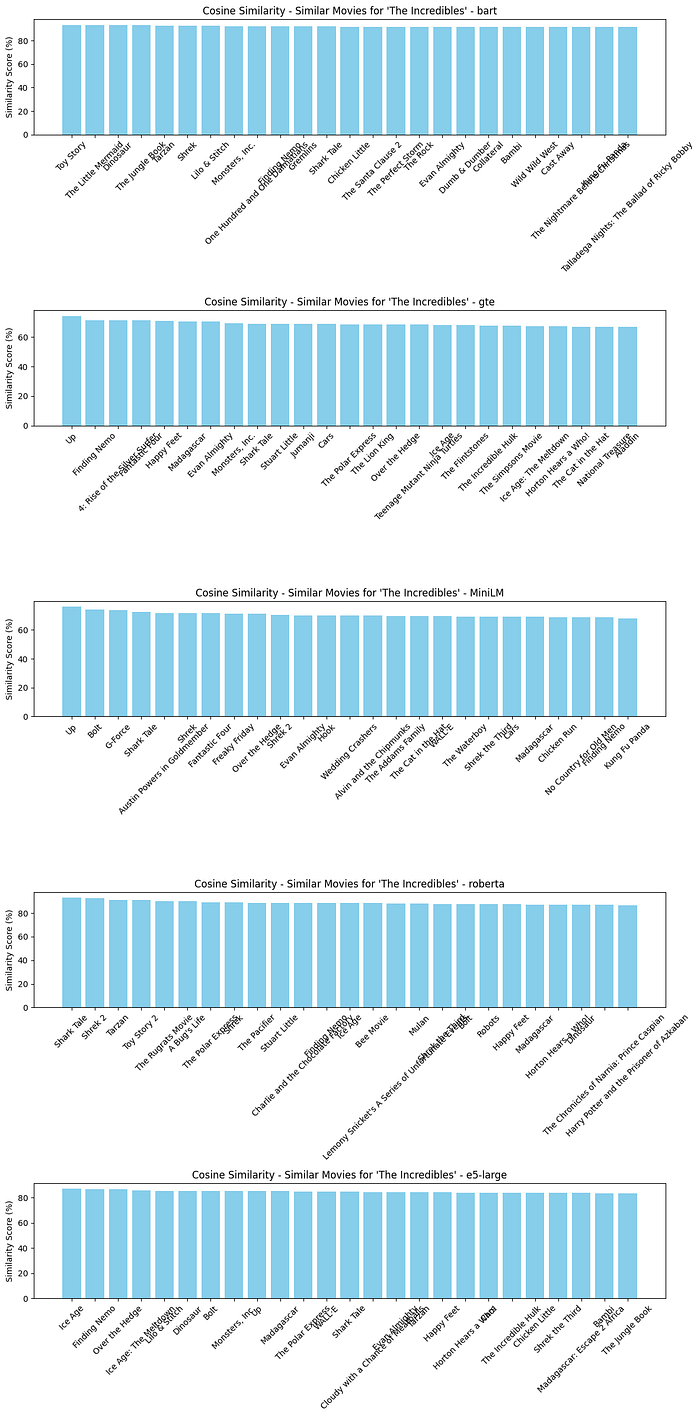
plot_compare_similar_movies_embedding([similar_movies_bart, similar_movies_gte, similar_movies_MiniLM, similar_movies_roberta, similar_movies_e5_large], “Cosine Similarity”)

Python

# For cosine similarity
similar_movies_cosine_bart = find_similar_movies(query_movie_title, threshold=0, distance_function=‘cosine_similarity’, embedding_type=‘bart’)
similar_movies_cosine_gte = find_similar_movies(query_movie_title, threshold=0, distance_function=‘cosine_similarity’, embedding_type=‘gte’)
similar_movies_cosine_MiniLM = find_similar_movies(query_movie_title, threshold=0, distance_function=‘cosine_similarity’, embedding_type=‘MiniLM’)
similar_movies_cosine_roberta = find_similar_movies(query_movie_title, threshold=0, distance_function=‘cosine_similarity’, embedding_type=‘roberta’)
similar_movies_cosine_e5_large = find_similar_movies(query_movie_title, threshold=0, distance_function=‘cosine_similarity’, embedding_type=‘e5_large’)
plot_compare_similar_movies_embedding([similar_movies_cosine_bart, similar_movies_cosine_gte, similar_movies_cosine_MiniLM, similar_movies_cosine_roberta, similar_movies_cosine_e5_large], “Cosine Similarity”)

# For L2 Distance (Euclidean Distance)
similar_movies_l2_bart = find_similar_movies(query_movie_title, threshold=0, distance_function=‘euclidean_distance’, embedding_type=‘bart’)
similar_movies_l2_gte = find_similar_movies(query_movie_title, threshold=0, distance_function=‘euclidean_distance’, embedding_type=‘gte’)
similar_movies_l2_MiniLM = find_similar_movies(query_movie_title, threshold=0, distance_function=‘euclidean_distance’, embedding_type=‘MiniLM’)
similar_movies_l2_roberta = find_similar_movies(query_movie_title, threshold=0, distance_function=‘euclidean_distance’, embedding_type=‘roberta’)
similar_movies_l2_e5_large = find_similar_movies(query_movie_title, threshold=0, distance_function=‘euclidean_distance’, embedding_type=‘e5_large’)
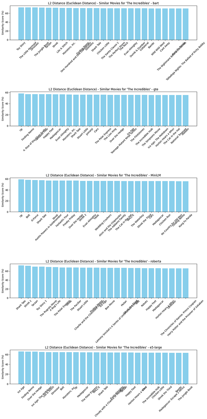
plot_compare_similar_movies_embedding([similar_movies_l2_bart, similar_movies_l2_gte, similar_movies_l2_MiniLM, similar_movies_l2_roberta, similar_movies_l2_e5_large], “L2 Distance (Euclidean Distance)”)

# For Inner Product
similar_movies_inner_bart = find_similar_movies(query_movie_title, threshold=0, distance_function=‘inner_product’, embedding_type=‘bart’)
similar_movies_inner_gte = find_similar_movies(query_movie_title, threshold=0, distance_function=‘inner_product’, embedding_type=‘gte’)
similar_movies_inner_MiniLM = find_similar_movies(query_movie_title, threshold=0, distance_function=‘inner_product’, embedding_type=‘MiniLM’)
similar_movies_inner_roberta = find_similar_movies(query_movie_title, threshold=0, distance_function=‘inner_product’, embedding_type=‘roberta’)
similar_movies_inner_e5_large = find_similar_movies(query_movie_title, threshold=0, distance_function=‘inner_product’, embedding_type=‘e5_large’)
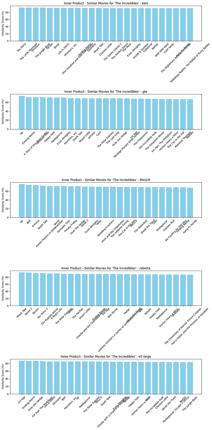
plot_compare_similar_movies_embedding([similar_movies_inner_bart, similar_movies_inner_gte, similar_movies_inner_MiniLM, similar_movies_inner_roberta, similar_movies_inner_e5_large], “Inner Product”)

# For Jaccard Distance
similar_movies_jaccard_bart = find_similar_movies(query_movie_title, threshold=0, distance_function=‘jaccard_distance’, embedding_type=‘bart’)
similar_movies_jaccard_gte = find_similar_movies(query_movie_title, threshold=0, distance_function=‘jaccard_distance’, embedding_type=‘gte’)
similar_movies_jaccard_MiniLM = find_similar_movies(query_movie_title, threshold=0, distance_function=‘jaccard_distance’, embedding_type=‘MiniLM’)
similar_movies_jaccard_roberta = find_similar_movies(query_movie_title, threshold=0, distance_function=‘jaccard_distance’, embedding_type=‘roberta’)
similar_movies_jaccard_e5_large = find_similar_movies(query_movie_title, threshold=0, distance_function=‘jaccard_distance’, embedding_type=‘e5_large’)
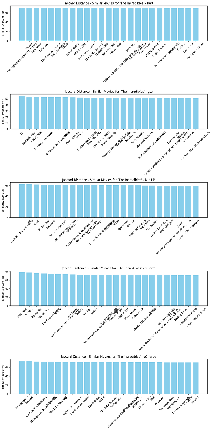
plot_compare_similar_movies_embedding([similar_movies_jaccard_bart, similar_movies_jaccard_gte, similar_movies_jaccard_MiniLM, similar_movies_jaccard_roberta, similar_movies_jaccard_e5_large], “Jaccard Distance”)

Comparing Different Embeddings

Using Pandas for Comparison for most similar movies

import pandas as pd
most_similar_movie_bart = find_similar_movies_sql(query_movie_title, threshold=0, return_n=1, distance_function=’<=>’, embedding_type=‘bart’)[0]
most_similar_movie_gte = find_similar_movies_sql(query_movie_title, threshold=0, return_n=1, distance_function=’<=>’, embedding_type=‘gte’)[0]
most_similar_movie_MiniLM = find_similar_movies_sql(query_movie_title, threshold=0, return_n=1, distance_function=’<=>’, embedding_type=‘MiniLM’)[0]
most_similar_movie_roberta = find_similar_movies_sql(query_movie_title, threshold=0, return_n=1, distance_function=’<=>’, embedding_type=‘roberta’)[0]
most_similar_movie_e5_large = find_similar_movies_sql(query_movie_title, threshold=0, return_n=1, distance_function=’<=>’, embedding_type=‘e5_large’)[0]
most_similar_movie_df = pd.DataFrame({
‘Title’: [most_similar_movie_bart[0], most_similar_movie_gte[0], most_similar_movie_MiniLM[0], most_similar_movie_roberta[0], most_similar_movie_e5_large[0]],
‘Similarity Score (%)’: [round(most_similar_movie_bart[1] * 100, 3), round(most_similar_movie_gte[1] * 100, 3), round(most_similar_movie_MiniLM[1] * 100, 3), round(most_similar_movie_roberta[1] * 100, 3), round(most_similar_movie_e5_large[1] * 100, 3)]
}, index=list(models.keys()))
print(most_similar_movie_df)

Title Similarity Score (%)
bart Toy Story 93.451
gte Up 74.388
MiniLM Up 75.960
roberta Shark Tale 92.904
e5-large Ice Age 86.908

Finding the Median Similar Movie

# find the most similar movie median
def find_most_similar_movie_median(title, threshold=0, distance_function=’<->’, embedding_type=‘bart’, n=631):
similar_movies = find_similar_movies_sql(title, threshold, n, distance_function, embedding_type)
if similar_movies:
similarities = [sim for _, sim in similar_movies]
# find median and return index
median_index = np.argsort(similarities)[len(similarities) // 2]
return similar_movies[median_index]
else:
return None

most_similar_movie_median_bart = find_most_similar_movie_median(query_movie_title, threshold=0, distance_function=’<=>’, embedding_type=‘bart’)
most_similar_movie_median_gte = find_most_similar_movie_median(query_movie_title, threshold=0, distance_function=’<=>’, embedding_type=‘gte’)
most_similar_movie_median_MiniLM = find_most_similar_movie_median(query_movie_title, threshold=0, distance_function=’<=>’, embedding_type=‘MiniLM’)
most_similar_movie_median_roberta = find_most_similar_movie_median(query_movie_title, threshold=0, distance_function=’<=>’, embedding_type=‘roberta’)
most_similar_movie_median_e5_large = find_most_similar_movie_median(query_movie_title, threshold=0, distance_function=’<=>’, embedding_type=‘e5_large’)

most_similar_movie_median_df = pd.DataFrame({
‘Title’: [most_similar_movie_median_bart[0], most_similar_movie_median_gte[0], most_similar_movie_median_MiniLM[0], most_similar_movie_median_roberta[0], most_similar_movie_median_e5_large[0]],
‘Similarity Score (%)’: [round(most_similar_movie_median_bart[1] * 100, 3), round(most_similar_movie_median_gte[1] * 100, 3), round(most_similar_movie_median_MiniLM[1] * 100, 3), round(most_similar_movie_median_roberta[1] * 100, 3), round(most_similar_movie_median_e5_large[1] * 100, 3)]
}, index=list(models.keys()))
print(most_similar_movie_median_df)

Title Similarity Score (%)
bart 101 Dalmatians 87.738
gte Blades of Glory 57.274
MiniLM The Bourne Ultimatum 52.563
roberta Speed 75.812
e5-large Titanic 78.170

Find the least similar movie

# find the least similar movie
def find_least_similar_movie(title, threshold=0.1, distance_function=’<->’, embedding_type=‘bart’, return_n=631):
similar_movies = find_similar_movies_sql(title, threshold, return_n, distance_function, embedding_type)
if similar_movies:
return similar_movies[-1]
else:
return None

least_similar_movie_bart = find_least_similar_movie(query_movie_title, threshold=0, distance_function=’<=>’, embedding_type=‘bart’)
least_similar_movie_gte = find_least_similar_movie(query_movie_title, threshold=0, distance_function=’<=>’, embedding_type=‘gte’)
least_similar_movie_MiniLM = find_least_similar_movie(query_movie_title, threshold=0, distance_function=’<=>’, embedding_type=‘MiniLM’)
least_similar_movie_roberta = find_least_similar_movie(query_movie_title, threshold=0, distance_function=’<=>’, embedding_type=‘roberta’)
least_similar_movie_e5_large = find_least_similar_movie(query_movie_title, threshold=0, distance_function=’<=>’, embedding_type=‘e5_large’)
least_similar_movie_df = pd.DataFrame({
‘Title’: [least_similar_movie_bart[0], least_similar_movie_gte[0], least_similar_movie_MiniLM[0], least_similar_movie_roberta[0], least_similar_movie_e5_large[0]],
‘Similarity Score (%)’: [round(least_similar_movie_bart[1] * 100, 3), round(least_similar_movie_gte[1] * 100, 3), round(least_similar_movie_MiniLM[1] * 100, 3), round(least_similar_movie_roberta[1] * 100, 3), round(least_similar_movie_e5_large[1] * 100, 3)]
}, index=list(models.keys()))
print(least_similar_movie_df)

Title Similarity Score (%)
bart Il buono, il brutto, il cattivo. 61.033
gte The Lady Vanishes 42.767
MiniLM Le notti di Cabiria 9.650
roberta Smultronstället 52.263
e5-large Ladri di biciclette 68.094

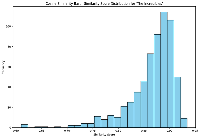
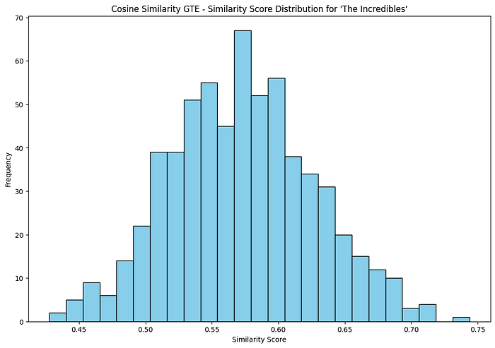
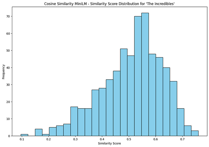
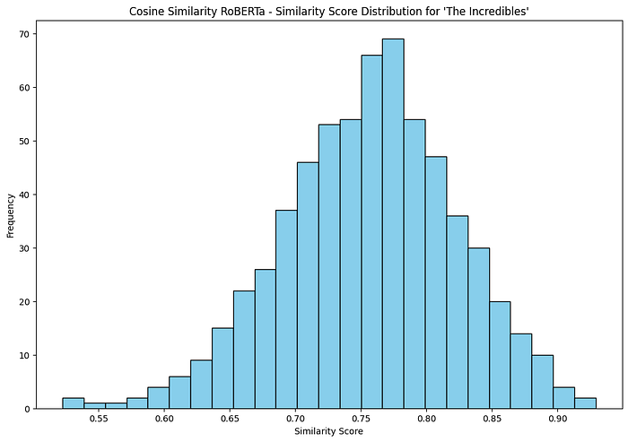
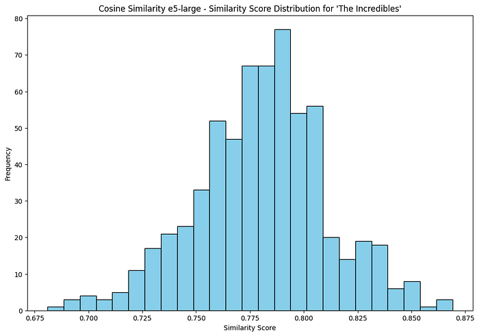
Show Distribution of Similarity Scores

def plot_similarity_distribution(similar_movies, title):
similarities = [sim[1] for sim in similar_movies]
plt.figure(figsize=(12, 8))
plt.hist(similarities, bins=25, color=‘skyblue’, edgecolor=‘black’)
plt.xlabel(‘Similarity Score’)
plt.ylabel(‘Frequency’)
plt.title(f"{title} - Similarity Score Distribution for ‘{query_movie_title}’")
plt.show()

similar_movies_bart = find_similar_movies_sql(query_movie_title, threshold=0, return_n=631, distance_function=’<=>’, embedding_type=‘bart’)
similar_movies_gte = find_similar_movies_sql(query_movie_title, threshold=0, return_n=631, distance_function=’<=>’, embedding_type=‘gte’)
similar_movies_MiniLM = find_similar_movies_sql(query_movie_title, threshold=0, return_n=631, distance_function=’<=>’, embedding_type=‘MiniLM’)
similar_movies_roberta = find_similar_movies_sql(query_movie_title, threshold=0, return_n=631, distance_function=’<=>’, embedding_type=‘roberta’)
similar_movies_e5_large = find_similar_movies_sql(query_movie_title, threshold=0, return_n=631, distance_function=’<=>’, embedding_type=‘e5_large’)

plot_similarity_distribution(similar_movies_bart, ‘Cosine Similarity Bart’)
plot_similarity_distribution(similar_movies_gte, ‘Cosine Similarity GTE’)
plot_similarity_distribution(similar_movies_MiniLM, ‘Cosine Similarity MiniLM’)
plot_similarity_distribution(similar_movies_roberta, ‘Cosine Similarity RoBERTa’)
plot_similarity_distribution(similar_movies_e5_large, ‘Cosine Similarity e5-large’)

Part 2 — Qdrant, MovieLens, and dense + sparse vectors

Above we stored dense movie embeddings in PostgreSQL and ran nearest-neighbor search in SQL. Here we use the same core idea—similarity in vector space—with Qdrant and MovieLens, and add a second mode that is not about text semantics: sparse vectors built from user ratings for collaborative-style recommendations.

The code described here comes from a small FastAPI teaching project (movie_recommendation): seed scripts under app/seed/ (for example load_movielens_100k_to_qdrant.py and load_movielens_1m_to_qdrant.py) load MovieLens into Qdrant collections; the API uses app/services/recommend.py, app/utils/embedding.py, and app/services/qdrant.py.

Three collections (MovieLens 100K example)

The 100K loader creates:

• movielens_100k_movies — dense vectors (384 dimensions, cosine) for semantic search over movie text.
• movielens_100k_users — dense user profiles (same embedding space as used in the seed pipeline).
• movielens_100k_ratings — sparse vectors named ratings: each dimension is a movie id, each value is a rating, so a user is a sparse vector over items they rated.

That split is the main design lesson: one engine (Qdrant), two different vector “meanings.”

Dense path: “something like this title”

create_embedding in app/utils/embedding.py uses sentence-transformers/all-MiniLM-L6-v2: tokenize, mean-pool the last hidden state, return a single embedding. For a query string, the service preprocesses text, embeds it, and calls client.search on the movies collection with query_vector as a plain dense vector.

Conceptually this matches Part 1: encode text → nearest movies by cosine similarity—only the storage and API are Qdrant instead of pgvector.

Sparse path: users like you

recommend_movies builds a NamedSparseVector: indices are movie ids, values are the user’s ratings. Qdrant searches the {prefix}_ratings collection (the seed script registers the sparse vector under the name ratings). Neighbors are similar users in rating space. The app then aggregates those neighbors’ ratings for movies the current user has not rated and returns top-scoring titles (resolving ids via a scroll over the movies collection).

So the second mode is collaborative filtering expressed as vector search—not retrieval from plot summaries, but from overlapping taste.

FastAPI surface

app/main.py mounts routers that expose these flows to a simple HTML UI. The interesting logic for readers of this post is in the service layer: dense search vs sparse neighbor aggregation.

Where to start in the SimilityVectorEmbedding course repo

If you are working through AlgoETS/SimilityVectorEmbedding in parallel, the qdrant/0.simple.ipynb notebook is the minimal Qdrant + movies.json exercise; it sits alongside the PostgreSQL track and matches the mental model “embed documents, upsert, query” before you add MovieLens scale and hybrid sparse+dense patterns.

Qdrant summary

• Similar movies by text: dense embeddings and cosine search on a movies collection.
• Similar taste: sparse rating vectors, nearest users in rating space, then aggregate their ratings for unseen items.

Qdrant adds a convenient way to mix dense and sparse vectors in one system alongside the pgvector workflow in Part 1.

Part 3 — Grounding movie Q&A with LangChain, Ollama, and pgvector

The same rows you load in Part 1 can back a small retrieve-then-generate flow: embed the user’s question, pull the nearest movies in SQL, then let a local LLM explain the hits with LangChain and Ollama. The reference notebook is postgres/3.LLMS.ipynb in AlgoETS/SimilityVectorEmbedding.

Why not only a general-purpose chat model?

A prompt like “movies similar to The Incredibles” against the open web does not guarantee answers from your catalog. The notebook contrasts that with answers constrained to rows in your movies table—the same idea as RAG: ground the model in evidence you control.

Pipeline at a glance

flowchart LR
  Q[User question] --> E[HuggingFaceEmbeddings]
  E --> SQL[SQL with pgvector kNN]
  SQL --> Rows[Top movie rows]
  Rows --> LLM[Ollama LLM via LangChain]
  LLM --> A[Natural language answer]

Retrieval: question to SQL + vectors

1. Embedding the question — HuggingFaceEmbeddings with sentence-transformers/all-MiniLM-L12-v2 (embed_query).
2. Similarity in SQL — The notebook builds a query that orders by cosine-style distance on embedding_MiniLM, e.g. using the pgvector <=> operator and 1 - (embedding_MiniLM <=> ARRAY[...]::vector) AS cosine_similarity, with ORDER BY cosine_similarity DESC and LIMIT 5.

This mirrors Part 1: same vectors and <=> idea, but the query vector comes from free text instead of an existing movie row.

Generation: schema-aware prompting + Ollama

The notebook wires LangChain: a ChatPromptTemplate describes the movies table (including embedding columns), asks for PostgreSQL-friendly behavior, and instructs the model to return question, SQL, formatted results, and a short natural-language answer. The runnable chain uses Ollama(model="llama2:13b-chat") and StrOutputParser().

ConversationBufferMemory is created in the notebook; the demonstrated flow is still essentially one-shot invocations per question.

What goes wrong in practice (and why it matters)

The saved notebook output is useful because it is messy:

• SQLAlchemy / LangChain warns that it does not recognize the vector type on embedding columns when reflecting the schema.
• The LLM sometimes emits SQL that does not match pgvector semantics (for example treating embeddings like scalars with @> or ANY(...) in ways that are not valid for your schema).
• Ollama can time out under load (llama2:13b-chat is heavy); one of the parallel test questions fails with a runner timeout.

Those issues are normal teaching points: RAG is not only “embed and search”—you need validation, fallbacks, smaller models, or hybrid retrieval when the generator drifts from executable SQL.

Running Part 3 yourself

You need PostgreSQL with pgvector, movie rows populated as in Part 1 above, Ollama with the chosen model pulled, and the Python stack from the notebook (langchain, langchain-community, langchain-huggingface, psycopg2, etc.). Adjust connection strings and model names to match your environment.

Conclusion

pgvector (Part 1) gives you transparent SQL and metrics over movie embeddings; Qdrant with MovieLens (Part 2) shows dense semantic search and sparse collaborative-style vectors in one engine; LangChain + Ollama (Part 3) shows how that same catalog becomes retrieval for grounded natural-language answers. Together they cover vector search, recommender-style signals, and a minimal RAG stack you can reproduce from the course repo.

Dataset reference: movies.json in SimilityVectorEmbedding.

The PostgreSQL / pgvector sections were originally published on Medium; this page also includes the Qdrant + MovieLens material and the LangChain + Ollama RAG notebook in one place.