Predicting Stock Prices with Monte Carlo Simulations

May 14, 2024

Introduction

In finance, decisions are rarely about a single “forecast” price: they are about ranges, tail risk, and how wrong simple models can be. This article walks through a Monte Carlo path simulation in Python: we estimate drift and volatility from historical closes, simulate many future price paths (a geometric Brownian–style discrete step), and summarize the result as a distribution—the right object for risk-style questions (bands, percentiles, coverage against a hold-out period).

Markov chain Monte Carlo (MCMC), as in Landauskas and Valakevičius’s paper on stock price modelling, is a different tool: it draws samples from a distribution that need not be a simple Gaussian—for example one built from a kernel density estimate of observed prices—whereas the code below assumes lognormal shocks from estimated drift and volatility. A practical workflow is MCMC (or other inference) for the law of the data, then forward Monte Carlo for multi-step scenarios. This post implements the forward GBM-style step explicitly; see the references and the linked work-in-progress below if you want to push toward paper-style MCMC.

Step 1: Setting Up the Environment

To start, we need to install the necessary Python libraries. These libraries include pandas, numpy, httpx, backtesting, pandas_ta, matplotlib, scipy, rich, and others. Here’s how to install them:

import pandas as pd
import numpy as np
from datetime import datetime
import concurrent.futures
import warnings
from rich.progress import track
from backtesting import Backtest, Strategy
import pandas_ta as ta
import matplotlib.pyplot as plt
from scipy.stats import norm
import httpx

warnings.filterwarnings(“ignore”)

Step 2: Defining Utility Functions

We need functions to fetch historical stock prices and crypto prices from APIs:

def make_api_request(api_endpoint, params):
with httpx.Client() as client:
# Make the GET request to the API
response = client.get(api_endpoint, params=params)
if response.status_code == 200:
return response.json()
print(“Error: Failed to retrieve data from API”)
return None

def get_historical_price_full_crypto(symbol):
api_endpoint = f"{BASE_URL_FMP}/historical-price-full/crypto/{symbol}"
params = {“apikey”: FMP_API_KEY}
return make_api_request(api_endpoint, params)

def get_historical_price_full_stock(symbol):
api_endpoint = f"{BASE_URL_FMP}/historical-price-full/{symbol}"
params = {“apikey”: FMP_API_KEY}

return make\_api\_request(api\_endpoint, params)

def get_SP500():
api_endpoint = “https://en.wikipedia.org/wiki/List_of_S%26P_500_companies”
data = pd.read_html(api_endpoint)
return list(data[0][‘Symbol’])

def get_all_crypto():
return [
“BTCUSD”, “ETHUSD”, “LTCUSD”, “BCHUSD”, “XRPUSD”, “EOSUSD”,
“XLMUSD”, “TRXUSD”, “ETCUSD”, “DASHUSD”, “ZECUSD”, “XTZUSD”,
“XMRUSD”, “ADAUSD”, “NEOUSD”, “XEMUSD”, “VETUSD”, “DOGEUSD”,
“OMGUSD”, “ZRXUSD”, “BATUSD”, “USDTUSD”, “LINKUSD”, “BTTUSD”,
“BNBUSD”, “ONTUSD”, “QTUMUSD”, “ALGOUSD”, “ZILUSD”, “ICXUSD”,
“KNCUSD”, “ZENUSD”, “THETAUSD”, “IOSTUSD”, “ATOMUSD”, “MKRUSD”,
“COMPUSD”, “YFIUSD”, “SUSHIUSD”, “SNXUSD”, “UMAUSD”, “BALUSD”,
“AAVEUSD”, “UNIUSD”, “RENBTCUSD”, “RENUSD”, “CRVUSD”, “SXPUSD”,
“KSMUSD”, “OXTUSD”, “DGBUSD”, “LRCUSD”, “WAVESUSD”, “NMRUSD”,
“STORJUSD”, “KAVAUSD”, “RLCUSD”, “BANDUSD”, “SCUSD”, “ENJUSD”,
]

def get_financial_statements_lists():
api_endpoint = f"{BASE_URL_FMP}/financial-statement-symbol-lists"
params = {“apikey”: FMP_API_KEY}
return make_api_request(api_endpoint, params)

Step 3: Splitting Data into Training and Testing Sets

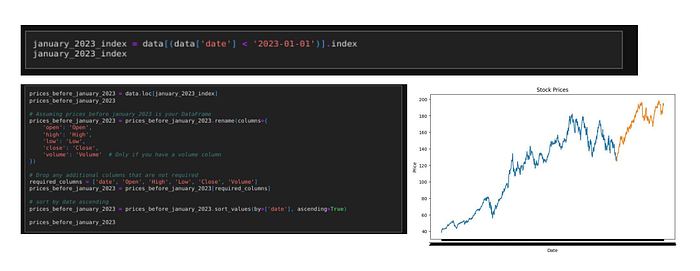
Next, we’ll fetch the historical stock prices for a given symbol and split the data into training and testing sets. We keep two frames: before January 2023 (used to estimate the model and run simulations) and from January 2023 onward (hold-out for comparing simulated ranges to realized prices).

stock_symbol = “AAPL”
stock_prices = get_historical_price_full_stock(stock_symbol)
data = pd.DataFrame(stock_prices[‘historical’])

def prepare_price_frame(df):
df = df.rename(columns={
‘open’: ‘Open’,
‘high’: ‘High’,
’low’: ‘Low’,
‘close’: ‘Close’,
‘volume’: ‘Volume’,
})
required_columns = [‘date’, ‘Open’, ‘High’, ‘Low’, ‘Close’, ‘Volume’]
return df[required_columns].sort_values(by=[‘date’], ascending=True).reset_index(drop=True)

prices_before_january_2023 = prepare_price_frame(data[data[‘date’] < ‘2023-01-01’])
prices_after_january_2023 = prepare_price_frame(data[data[‘date’] >= ‘2023-01-01’])

plt.figure(figsize=(10, 6))
plt.title(‘Stock Prices’)
plt.xlabel(‘Date’)
plt.ylabel(‘Price’)
plt.plot(prices_before_january_2023[‘date’], prices_before_january_2023[‘Close’], label=‘Train (before Jan 2023)’)
plt.plot(prices_after_january_2023[‘date’], prices_after_january_2023[‘Close’], label=‘Hold-out (from Jan 2023)’)
plt.legend()
plt.show()

Press enter or click to view image in full size

Step 4: Monte Carlo Simulation (Forward Paths and Risk Bands)

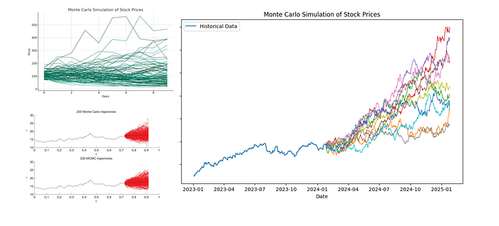
The function below is Monte Carlo simulation of a constant-parameter model: we estimate mean and variance of log returns on the training window, build a daily drift and volatility, then draw many independent Gaussian shocks and propagate price forward. That is not MCMC; there is no Markov chain sampling a posterior here. It is the kind of forward scenario engine you might run after inference. By contrast, Landauskas and Valakevičius (Intellectual Economics, 2011) use MCMC to sample from a distribution shaped by a kernel density estimate of prices (piecewise-linear proposals)—a way to stay close to the empirical law of the data with few parametric assumptions. Our GBM shortcut is simpler; the paper is the reference when you want the data-driven sampling step.

For a work-in-progress that extends this line of thought (batch experiments, richer risk views, and moving closer to paper-style MCMC), see this LinkedIn experiment (WIP).

The useful outputs for risk are distributions: percentiles of terminal price, prediction-style bands (for example 5th–95th percentile paths), and coverage checks against a hold-out (did realized prices sit where the simulated mass was?).

def monte_carlo_simulation(data, days, iterations):
if isinstance(data, pd.Series):
data = data.to_numpy()
if not isinstance(data, np.ndarray):
raise TypeError(“Data must be a numpy array or pandas Series”)

log\_returns = np.log(data\[1:\] / data\[:-1\])  
mean = np.mean(log\_returns)  
variance = np.var(log\_returns)  
drift = mean - (0.5 \* variance)  
daily\_volatility = np.std(log\_returns)  

future\_prices = np.zeros((days, iterations))  
current\_price = data\[-1\]  
for t in range(days):  
    shocks = drift + daily\_volatility \* norm.ppf(np.random.rand(iterations))  
    future\_prices\[t\] = current\_price \* np.exp(shocks)  
    current\_price = future\_prices\[t\]  
return future\_prices

Press enter or click to view image in full size

Visualisation

simulation_days = 364
mc_iterations = 1000
mc_prices = monte_carlo_simulation(prices_before_january_2023[‘Close’], simulation_days, mc_iterations)

last_train_close = prices_before_january_2023[‘Close’].iloc[-1]
last_close_price = np.full((1, mc_iterations), last_train_close)
mc_prices_combined = np.concatenate((last_close_price, mc_prices), axis=0)

last_date = prices_before_january_2023[‘date’].iloc[-1]
simulated_dates = pd.date_range(start=last_date, periods=simulation_days + 1)

# Percentiles across paths at each future step (risk band)
p05 = np.percentile(mc_prices_combined, 5, axis=1)
p50 = np.percentile(mc_prices_combined, 50, axis=1)
p95 = np.percentile(mc_prices_combined, 95, axis=1)
mean_path = mc_prices_combined.mean(axis=1)

# Terminal distribution at the last simulated step (VaR-style summaries)
terminal_prices = mc_prices_combined[simulation_days, :]
mean_terminal_price = float(np.mean(terminal_prices))
q5, q50, q95 = np.percentile(terminal_prices, [5, 50, 95])
terminal_return = terminal_prices / last_train_close - 1.0
ret_q5, ret_q50, ret_q95 = np.percentile(terminal_return, [5, 50, 95])

horizon_idx = min(simulation_days, len(prices_after_january_2023) - 1)
real_price = float(prices_after_january_2023[‘Close’].iloc[horizon_idx])
real_date = prices_after_january_2023[‘date’].iloc[horizon_idx]
in_90_band = q5 <= real_price <= q95

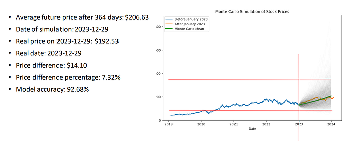
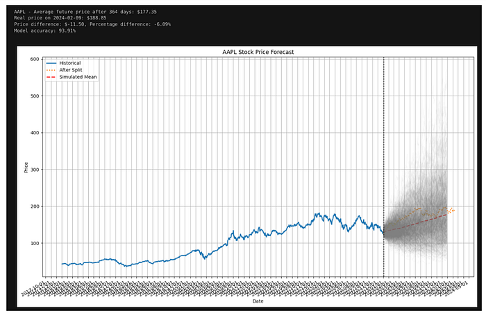
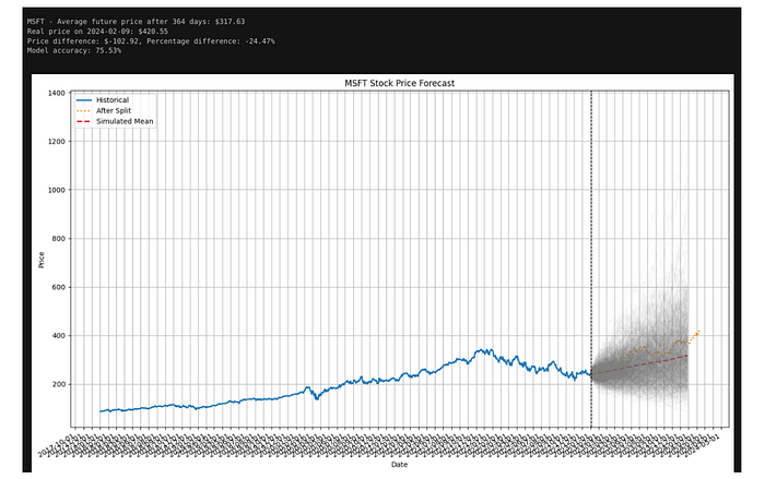
print(f"Simulated horizon: {simulation_days} trading days after {last_date}")
print(f"Mean terminal price: ${mean_terminal_price:.2f}")
print(f"Terminal price percentiles (5 / 50 / 95): ${q5:.2f} / ${q50:.2f} / ${q95:.2f}")
print(f"Terminal simple return vs last train close — 5th / 50th / 95th %ile: {ret_q5*100:.2f}% / {ret_q50*100:.2f}% / {ret_q95*100:.2f}%")
print(f"Hold-out price at aligned step ({real_date}): ${real_price:.2f}")
print(f"Realized price inside simulated 5–95% band: {in_90_band}")

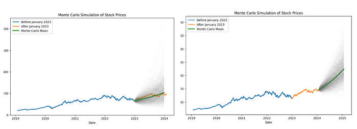
plt.figure(figsize=(10, 6))
for i in range(mc_iterations):
plt.plot(simulated_dates, mc_prices_combined[:, i], linewidth=0.5, color=‘gray’, alpha=0.02)
plt.fill_between(simulated_dates, p05, p95, alpha=0.25, label=‘5th–95th percentile band’)
plt.plot(simulated_dates, p50, label=‘Median path’, linewidth=2, color=‘C0’)
plt.plot(simulated_dates, mean_path, label=‘Mean path’, linewidth=2, linestyle=’–’, color=‘C1’)
plt.plot(pd.to_datetime(prices_before_january_2023[‘date’]), prices_before_january_2023[‘Close’], label=‘Train (before Jan 2023)’, linewidth=2, color=‘black’)
plt.plot(pd.to_datetime(prices_after_january_2023[‘date’]), prices_after_january_2023[‘Close’], label=‘Hold-out (from Jan 2023)’, linewidth=2, color=‘green’)
plt.axvline(pd.to_datetime(real_date), color=‘red’, linestyle=’:’, linewidth=1, alpha=0.8, label=‘Hold-out step aligned to horizon’)
plt.scatter([pd.to_datetime(real_date)], [real_price], color=‘red’, s=40, zorder=5, label=‘Realized (aligned)’)

plt.title(‘Monte Carlo Simulation of Stock Prices (with percentile band)’)
plt.xlabel(‘Date’)
plt.ylabel(‘Price’)
plt.legend(loc=‘upper left’, fontsize=8)
plt.show()

Press enter or click to view image in full size

Conclusion

Forward Monte Carlo gives you a distribution of future prices under an assumed dynamics—ideal for percentile bands, tail behaviour, and coverage checks against data you held out. That is a different step from MCMC, which is about sampling from a flexible model of the data (as in Landauskas and Valakevičius’s KDE-driven approach) before or alongside forward simulation. A practical pipeline is: fit or sample the distribution that matches history, then push scenarios forward with Monte Carlo. Combined with strategy backtesting, you separate “how wide is model risk?” from “does a rule make money?”

Related exploratory code: AlgoETS/MarkokChainMonteCarlo (stratification / MCMC-oriented experiments).

Reference

Landauskas, M. & Valakevičius, E. (2011). Modelling of Stock Prices by Markov Chain Monte Carlo Method — Intellectual Economics, Vol. 5 No. 2 (article page); PDF download.
Semantic Scholar index for the same paper.
Neural Networks in Finance: Markov Chain Monte Carlo (MCMC) and Stochastic Volatility Modeling
Monte Carlo Simulation Basics

Originally published on Medium.